Hands On Machine Learning

2 End-to-End Machine Learning Project¶

Fine Tune Model¶

Grid Search¶

Search the hyperparameters manually is very tedious, GridSearchCV may search for you after tell it which hyperparameters you want it to experiment with, and what values to try out, and it will evaluate all the possible combinations of hyperparameter values, using cross-validation.

from sklearn.model_selection import GridSearchCV
param_grid = [
{'n_estimators': [3, 10, 30], 'max_features': [2, 4, 6, 8]}, 
{'bootstrap': [False], 'n_estimators': [3, 10], 'max_features': [2, 3, 4]}, 
]
forest_reg = RandomForestRegressor()
grid_search = GridSearchCV(forest_reg, param_grid, cv=5, 
                    scoring='neg_mean_squared_error')
grid_search.fit(housing_prepared, housing_labels)

Tip

When you have no idea what value a hyperparameter should have, a simple approach is to try out consecutive powers of 10 or a smaller number if you want a more fine-grained search.

6 Decision Trees¶

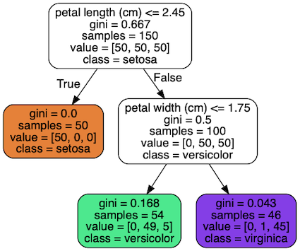
Classification¶

from sklearn.datasets import load_iris 
from sklearn.tree import DecisionTreeClassifier

iris = load_iris() 
# petal length and width 
X = iris.data[:, 2:] 
y = iris.target
tree_clf = DecisionTreeClassifier(max_depth=2) 
tree_clf.fit(X, y)
tree_clf.predict([[5, 1.5])

iris_tree

Cost Function¶

SkLearn uses the CART algorithm. CART cost function for classification is

$J(k, t_k) = \frac{m_{left}}{m}G_{left} + \frac{m_{right}}{m}G_{right}$

where $G_{left/right}$ measures the impurity of the left/right subset, and $m_{left/right}$ is the number of instances in the left/right subset.

The CART algorithm is a greedy algorithms: it greedily searches for an optimum split at the top level, then repeats the process at each level. It does not check whether or not the split will lead to the lowest possible impurity several levels down.

Finding the optimal tree is known to be an NP-Complete problem: it requires $O(\exp(m))$ time.

Computational Complexity¶

Predictions: $O(\log m)$ , where $m$ is the number of instances.
- traversing the tree from the root to a leaf, the height of the tree is $O(\log m)$ .
Training: $O(nm \log m)$ , where $n$ is the number of features.
- compares all features $n$ on all samples $m$ at every level of the tree.

Gini impurity or entropy¶

Most of the time it does not make a big difference: they lead to similar trees. Gini impurity is slightly faster to compute, so it is a good default. However, when they differ,

Gini impurity tends to isolate the most frequent class in its own branch of the tree
while entropy tends to produce slightly more balanced trees.

Regression¶

from sklearn.tree import DecisionTreeRegressor

tree_reg = DecisionTreeRegressor(max_depth=2)
tree_reg.fit(X, y)

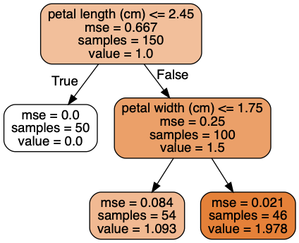
Cost Function¶

CART cost function for regression:

$J(k, t_k)= \frac{m_{left}}{m} \text{MSE}_{left} + \frac{m_{right}}{m}\text{MSE}_{right}$

Instability¶

Decision Trees love orthogonal decision boundaries, which makes them sensitive to training set rotation.

After the dataset is rotated by 45°, the decision boundary looks unnecessarily convoluted.

One way to limit this problem is to use PCA, which often results in a better orientation of the training data.

More generally, the main issue with Decision Trees is that they are very sensitive to small variations in the training data.