Relational Data

Pandas SQLite SQL

Overview of relational data

The term technical term “relation” can be interchanged with the standard notion we have of “tabular data,” say an instance of a “Person” relation:

Person

ID	Last Name	First Name	Role
1	Kolter	Zico	Instructor
2	Xi	Edgar	TA
3	Lee	Mark	TA
4	Mani	Shouvik	TA
5	Gates	Bill	Student
6	Musk	Elon	Student

• Rows are called tuples (元祖 or records), represent a single instance of this relation, and must be unique.
• Columns are called attributes(属性), specify some element contained by each of the tuples.
• Primary key(主键): an unique ID for every tuple in a relation (i.e. every row in the table), each relation must have exactly one primary key
• foreign key(外键): an attribute that points to the primary key of another relation
• Indexes(索引) are created as ways to “quickly” access elements of a table
  • In practice, use data structure like a B-tree or several others
  • searching for value takes $𝑂(\log 𝑛)$ time
  • Indexes don’t have to be on a single column, can have an index over multiple columns (with some ordering)

Entity relationships

The nature of inter-table relationships via primary and foreign keys actually leads to a number of different possible entity relationships(实体关系) (i.e., relationships between a row in one table and a row in another). Several types of inter-table relationships

1. One-to-one
2. (One-to-zero/one)
3. One-to-many (and many-to-one)
4. Many-to-many

These relate one (or more) rows in a table with one (or more) rows in another table, via a foreign key.

One-to-many relationship

We have already seen a one-to-many relationship: one role can be shared by many people, denoted as follows

Role

ID	Name
1	Instructor
2	TA
3	Student

One-to-one relationships

In a true one-to-one relationship spanning multiple tables, each row in a table has exactly one row in another table

Andrew ID

Person ID	Andrew ID
1	zkoler
2	esx
3	marklee
4	shouvikm
5	bgates
6	muskleman

One-to-zero/one relationships

More common in databases is to find “one-to-zero/one” relationships broken across multiple tables.

Consider adding a “Grades” table to our database: each person can have at most one tuple in the grades table.

Grades

Person ID	HW1 Grade	HW2 Grade
5	85	95
6	80	60

Many-to-many relationships

Alternatively, consider adding two tables, a “homework” table that represents information about each homework, and an associative table that links homeworks to people.

Homework

ID	Name	Points	Release Date	Due Date
1	HW1	100	2018-01-24	2018-02-07
2	HW2	100	2018-02-07	2018-02-21

Person Homework

Person ID	Homework ID	Score
5	1	85
5	2	95
6	1	80
6	2	60

Pandas

Pandas is a “Data Frame” library in Python, meant for manipulating in memory data with row and column labels (as opposed to, e.g., matrices, that have no row or column labels).

Pandas is not a relational database system, but it contains functions that mirror some functionality of relational databases.

Operations in Pandas are typically not in place (that is, they return a new modified DataFrame, rather than modifying an existing one). Use the inplace=True flag to make them done in place.

Create a DataFrame with our Person example:

import pandas as pd
df = pd.DataFrame([(1, 'Kolter', 'Zico'), 
                   (2, 'Xi', 'Edgar'),
                   (3, 'Lee', 'Mark'), 
                   (4, 'Mani', 'Shouvik'),
                   (5, 'Gates', 'Bill'),
                   (6, 'Musk', 'Elon')], 
                  columns=["id", "last_name", "first_name"])
df.set_index("Person ID", inplace=True)

If you select a single row or column in a Pandas DataFrame, this will return a Series object, which is like a one-dimensionalDataFrame (it has only an index and corresponding values, not multiple columns)

Common Pandas data access

You can access individual elements using the .loc[row, column] notation, where row denotes the index you are searching for and column denotes the column name.

# access the last name of person with ID 1
df.loc[1, "last_name"]  
# access all last names, return a Pandas Series
df.loc[:, "last_name"]  
# access all last name, return a Pandas DataFrame
df.loc[:, ['last_name']] 
# access last name of person with ID 1,2, return a DataFrame
df.loc[[1,2],:]
# change the last name of person with ID 1
df.loc[1,"last_name"] = "Kilter"
# Add a new entry with index=7 
df.loc[7,:] = ("Moore", "Andrew") 
# Index rows and columns by zero-index
df.iloc[0,0]

SQLite

SQLite is a full-featured database, but it does not use a client/server model. Databases are instead stored directly on disk and accessed just via the library. This has the advantage of being very simple, with no server to configure and run, but for large applications it is typically insufficient.

SQLite, as the name suggests, uses the SQL (structured query language) language for interacting with the database.

Creating a database and table

You can create a database and connect using this boilerplate code:

import sqlite3 
conn = sqlite3.connect("people.db") 
cursor = conn.cursor()
conn.close()

Create a new table:

cursor.execute(
""" CREATE TABLE role (
    id INTEGER PRIMARY KEY,
    name TEXT 
)""")

Creating a new table and inserting data

Insert data into the table:

cursor.execute("INSERT INTO role VALUES (1, 'Instructor')") 
cursor.execute("INSERT INTO role VALUES (2, 'TA')") 
cursor.execute("INSERT INTO role VALUES (3, 'Student')") 
conn.commit()

Delete items from a table:

cursor.execute("DELETE FROM role WHERE id == 3") 
conn.commit()

Pandas

Alternatively, it can be handy to dump the results of a query directly into a Pandas DataFrame. Fortunately, Pandas provides a nice call for doing this, the pd.read_sql_query() function, with takes the database connection and an optional argument to set the index of the Pandas Dataframe to be one of the columns.

pd.read_sql_query("SELECT * from person;", conn, index_col="id")

Joins

Join operations merge multiple tables into a single relation (can be then saved as a new table or just directly used). You join two tables on columns from each table, where these columns specify which rows are kept.

Four typical types of joins:

1. Inner
2. Left
3. Right
4. Outer

Inner Join

Join two tables where we only return the rows where the two joined columns contain the same value.

ID	Last Name	First Name	HW1 Grade	HW2 Grade
5	Gates	Bill	85	95
6	Musk	Elon	80	60

df_person = pd.read_sql_query("SELECT * FROM person", conn)
df_grades = pd.read_sql_query("SELECT * FROM grades", conn)
df_person.merge(df_grades, how="inner", left_on = "id", right_on="person_id")

If you alternatively want to join on the index for the left or right data frame, you specify the left_index or right_index parameters as so:

df_person.set_index("id", inplace=True)
df_grades.set_index("person_id", inplace=True)
df_person.merge(df_grades, how="inner", left_index=True, right_index=True)

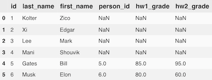
Left/Right Join

Whereas an inner join only kept those rows with corresponding entires in both tables, a left join will keep all the items in the left table, and add in the attribution from the right table (filling with NaNs if no match exists in the right table). Any row value that occurs in the right table but not the left table is discarded.

For the rest of this section, we'll simply write the Pandas code to perform the relevant join, then show the output it produces, rather than explicitly write the table that results.

df_person = pd.read_sql_query("SELECT * FROM person", conn)
df_grades = pd.read_sql_query("SELECT * FROM grades", conn)
df_person.merge(df_grades, how="left", left_on = "id", right_on="person_id")

Outer joins (also called a cross product) keep all rows that occur in either table, so essentially take the union of the left and right joins.

df_person.merge(df_grades, how="outer", left_on = "id", right_on="person_id")